45 excel pivot table conditional formatting row labels

trumpexcel.com › group-numbers-in-pivot-tableHow to Group Numbers in Pivot Table in Excel You May Also Like the Following Pivot Table Tutorials: How to Group Dates in Pivot Table in Excel. How to Create a Pivot Table in Excel. Preparing Source Data For Pivot Table. How to Refresh Pivot Table in Excel. Using Slicers in Excel Pivot Table – A Beginner’s Guide. How to Apply Conditional Formatting in a Pivot Table in Excel. Excel Conditional Formatting in Pivot Table - EDUCBA Click on any cell in the pivot table > Go to the HOME tab > Click on Conditional Formatting option under Styles option > Click on Manage Rules option. It will open a Rules Manager dialog box. Click on the Edit Rule tab, as shown in the below screenshot. It will open the Editing Rule formatting window. Refer to the below screenshot.

Excel Pivot Table Conditional Formatting Row Labels Go making the conditional formatting select the color scale and do it based on commercial and choose diverging and the colors should give expected result. Here a glaze color or bar and been applied...

Excel pivot table conditional formatting row labels

Using column label as formatting condition in excel pivot table I have pivot table in excel with sample data as attached. I now want to apply conditional formatting as red background where - data is between 10 to 25 AND - year is 2011 and 2012. =AND(C1="2011",OR(C2>10,C2<25)) how do i make cells example c2,c3,d2 red based on condition of year. Without Year condition it is working fine. Format Pivot Table Labels Based on Date Range Select all the dates in the Row Labels that you want to format. On the Ribbon, click the Home tab, and then in the Styles group, click Conditional Formatting. In the list of conditional formatting options, click Highlight Cells Rules, and then click A Date Occurring. Excel VBA: Conditional Format of Pivot Table based on Column Label myPivotSourceName = myPivotField.Name. Then rather than referencing the data field with the pivot field object, I referenced the DataRange with the string: myPivotTable.PivotFields (myPivotSourceName).DataRange.Select. Works perfectly and is completely portable for any pivottable on any sheet with any fields. excel vba.

Excel pivot table conditional formatting row labels. Design the layout and format of a PivotTable In the PivotTable Options dialog box, click the Layout & Format tab, and then under Layout, select or clear the Merge and center cells with labels check box. Note: You cannot use the Merge Cells check box under the Alignment tab in a PivotTable. Change the display of blank cells, blank lines, and errors Pivot Table with Conditional Formatting - Microsoft Community Ok, Pivot Tables are good, Pivot Tables are our friends. Now I want to use conditional formatting with a pivot table. I have seen a lot of examples, but none showing me how to use a field in the field list in the formula of a conditional format. Perhaps this is not possible, so I moved the field into a row label. › blog › insert-blank-rows-inHow to Insert a Blank Row in Excel Pivot Table - MyExcelOnline Jan 17, 2021 · STEP 1: Click any cell in the Pivot Table. STEP 2: Go to Design > Blank Rows. STEP 3: You will need to click on the Blank Rows button and select Insert Blank Line After Each Item. NB: For this to work you will need at least two Pivot Table Items in the Rows Labels. You then get the following Pivot Table report: Apply Conditional Formatting | Excel Pivot Table Tutorial Go to Home Tab → Styles → Conditional Formatting → New Rule. From rule to, select the third option. And, from "select a rule" type select "Format only top or bottom" ranked values. In edit rule description, enter 1 in the input box and from the drop-down menu select "each Column Group". Apply formatting you want. Click OK.

› pivot-table-tips-and-tricks101 Advanced Pivot Table Tips And Tricks You Need To Know Apr 25, 2022 · Without a table your range reference will look something like above. In this example, if we were to add data past Row 51 or Column I our pivot table would not include it in the results. To create and name your table. Select your data. Go to the Insert tab and press the Table button in the Tables section, or use the keyboard shortcut Ctrl + T. Conditional Format Pivot Table Row | Chandoo.org Excel Forums - Become ... Excel Ninja Apr 3, 2013 #2 Select the entire row, and when you apply the conditional format, make the column reference absolute. So, say we want the entire row 2 to be formatted if cell in col B = 5. formula would be: =$B2=5 How to make row labels on same line in pivot table? Make row labels on same line with PivotTable Options You can also go to the PivotTable Options dialog box to set an option to finish this operation. 1. Click any one cell in the pivot table, and right click to choose PivotTable Options, see screenshot: 2. › pivot-tables › pivot-tableHow to Apply Conditional Formatting to Pivot Tables - Excel ... Dec 13, 2018 · How to Setup Conditional Formatting for Pivot Tables. Setting up conditional formatting for pivot tables is a little different than it is for regular cells/ranges. So in this post I explain how to apply conditional formatting for pivot tables. 1. Select a cell in the Values area. The first step is to select a cell in the Values area of the ...

How to Apply Conditional Formatting in Pivot Table? (with ... To apply conditional formatting in the pivot table, first, we must select the column to format. In this example, select "Grand Total Column." Then, in the "Home" Tab in the "Styles" section, click on "Conditional Formatting." Consequently, a dialog box pops up. Then, we need to click on "New Rule." As a result, another dialog box will pop up. conditional formatting per row on pivot - Microsoft Tech ... conditional formatting per row on pivot. Hi, I would like to format each row of a pivot table separately (as in the picture shown below), but I cannot paste the formatting. I've got many rows, and they could change (just like the columns) Is there a way to automate this, or I have to select row by row and apply the formatting? Excel Pivot Table Conditional Formatting - XpCourse In short, Barreto creates a Pivot Table using "up to 8.5 million rows with no problem at all." The above image comes from the blog post, showing a total of 2 million rows in use in Excel. Remember, this process doesn't split the CSV into small chunks. ... excel pivot table conditional formatting provides a comprehensive and comprehensive ... › documents › excelHow to remove bold font of pivot table in Excel? - ExtendOffice The normal Bold feature can’t help us to un-bold the row labels in pivot table, but we can apply the powerful function – Conditional Formatting to solve this problem. Please do as follows: 1. Select the bold font row you want to un-bold in the pivot table, or you can press Ctrl key to select multiple bold font rows as your need. See screenshot:

How To Find And Remove Duplicates In A Pivot Table - MS Excel | Excel In Excel

Apply conditional formatting for each row in Excel Then click Format button, in the Format Cells dialog, under Fill tab, select green color. Click OK > OK. 4. Then drag the AutoFill handle to adjacent rows which you want to apply the conditional rule to, then in select Fill Formatting Only from the Auto Fill Options. Sample File Click to download the sample file

How To Sort A Table In Excel | Decoration Examples

Excel tutorial: How to highlight rows with conditional formatting To highlight rows in the table that contain tasks assigned to Bob, we need to take a different approach. First, select all of the data in the list. Then, choose New Rule from the conditional format menu on the Home tab of the ribbon. For style, choose "Classic". Then select "Use a formula to determine which cells to format".

Excel KPI Dashboard to Monitor Salesman

blog.hubspot.com › marketing › how-to-create-pivotHow to Create a Pivot Table in Excel: A Step-by-Step Tutorial Dec 31, 2021 · After you've completed Step 3, Excel will create a blank pivot table for you. Your next step is to drag and drop a field — labeled according to the names of the columns in your spreadsheet — into the Row Labels area. This will determine what unique identifier — blog post title, product name, and so on — the pivot table will organize ...

Learn Pivot Table - Tutorial & Magical Quotes: Easy way to Learn Pivot Table Step By Step ...

How to rename group or row labels in Excel PivotTable? To rename Row Labels, you need to go to the Active Field textbox. 1. Click at the PivotTable, then click Analyze tab and go to the Active Field textbox. 2. Now in the Active Field textbox, the active field name is displayed, you can change it in the textbox.

How to Apply Data Bars in Pivot Table - MS Excel | Excel In Excel

Pivot Table Conditional Formatting with VBA - Peltier Tech It seems to occur because in 2007, conditional format is applied to a field, whereas in 2003, it's applied to a range. Without resorting to macros, it's possible to quickly reapply the conditional format in 2007 by following these steps: - Set the conditional format to range covering more than the pivot table (e.g. on cell above).

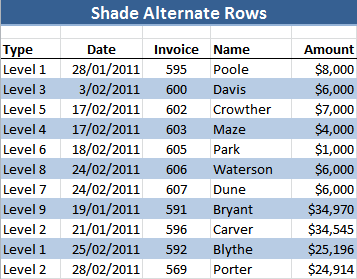
Excel Conditional Formatting Zebra Stripes • My Online Training Hub

Pivot Tables in Excel - Excel IF | No 1 Excel tutorial on the net Insert a Pivot Table. To insert a pivot table, execute the following steps. 1. Click any single cell inside the data set. 2. On the Insert tab, in the Tables group, click PivotTable. The following dialog box appears. Excel automatically selects the data for you. The default location for a new pivot table is New Worksheet.

microsoft office - Excel 2013 table formatting - Super User

Conditional formatting for Pivot Tables in Excel 2016 - Ablebits The format I used was to select Conditional Formatting > Top 10 Items > set it to 1 item and select the default format. This format can be copied from one range to the next if desired or built up for each range individually. To copy the format, select one or more cells with that format and click Copy.

How to Create a MS Excel Pivot Table – An Introduction | SIMPLE TAX INDIA

How to Apply Conditional Formatting to Rows Based on ... - Excel Campus On the Home tab of the Ribbon, select the Conditional Formatting drop-down and click on Manage Rules…. That will bring up the Conditional Formatting Rules Manager window. Click on New Rule. This will open the New Formatting Rule window. Under Select a Rule Type, choose Use a formula to determine which cells to format.