41 excel chart only show certain data labels
superuser.com › questions › 1195816Excel Chart not showing SOME X-axis labels - Super User Apr 05, 2017 · I was having a similar problem and it was only due to what excel can fit in the chart. Click the chart, and then drag one of the sizing handles to enlarge the chart. By default, the fonts in the chart scale proportionally as you resize the chart. Once you make your chart big enough, your labels should show. Add data labels to chart but only for most recent and ... For a new thread (1st post), scroll to Manage Attachments, otherwise scroll down to GO ADVANCED, click, and then scroll down to MANAGE ATTACHMENTS and click again. Now follow the instructions at the top of that screen. New Notice for experts and gurus:
How to Only Show Selected Data Points in an Excel Chart ... Download Free Sample Dashboard Files here: on how to show or hide specific data points i...

Excel chart only show certain data labels
Display Data Labels for only the First and Last Data ... Excel Questions Display Data Labels for only the First and Last Data Points 3link Mar 3, 2011 3 3link Board Regular Joined Oct 15, 2010 Messages 138 Mar 3, 2011 #1 My graph looks like this: Basically, I want to get rid of the center labels for the red and blue lines (series). This is a dynamic graph and the value will vary by user input. Only Label Specific Dates in Excel Chart Axis - Reduce ... Date axes can get cluttered when your data spans a large date range. Use this easy technique to only label specific dates.Download the Excel file here: https... Excel Chart - Do not Hide Horizontal Data Label - Stack ... 1) You can't see all your data labels on the X axis unless you format the X axis to have major interval of 1. 2) With a scatter plot, you cannot have your original labels retained on the X axis and, in your case, as your dates are recognised , they are ordered as such.
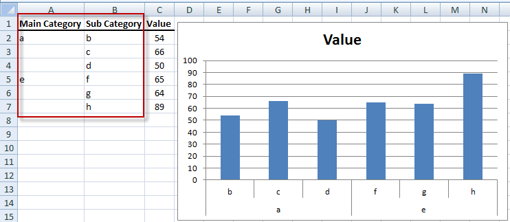
Excel chart only show certain data labels. peltiertech.com › prevent-overlapping-data-labelsPrevent Overlapping Data Labels in Excel Charts - Peltier Tech May 24, 2021 · Overlapping Data Labels. Data labels are terribly tedious to apply to slope charts, since these labels have to be positioned to the left of the first point and to the right of the last point of each series. This means the labels have to be tediously selected one by one, even to apply “standard” alignments. How to Use Cell Values for Excel Chart Labels Select the chart, choose the "Chart Elements" option, click the "Data Labels" arrow, and then "More Options." Uncheck the "Value" box and check the "Value From Cells" box. Select cells C2:C6 to use for the data label range and then click the "OK" button. The values from these cells are now used for the chart data labels. charts - Excel, giving data labels to only the top/bottom ... 1) Create a data set next to your original series column with only the values you want labels for (again, this can be formula driven to only select the top / bottom n values). See column D below. 2) Add this data series to the chart and show the data labels. 3) Set the line color to No Line, so that it does not appear! 4) Volia! See Below! Share Excel charts: add title, customize chart axis, legend and ... Click the Chart Elements button, and select the Data Labels option. For example, this is how we can add labels to one of the data series in our Excel chart: For specific chart types, such as pie chart, you can also choose the labels location. For this, click the arrow next to Data Labels, and choose the option you want.
support.microsoft.com › en-us › officeCreate a Map chart in Excel - support.microsoft.com Simply input a list of geographic values, such as country, state, county, city, postal code, and so on, then select your list and go to the Data tab > Data Types > Geography. Excel will automatically convert your data to a geography data type, and will include properties relevant to that data that you can display in a map chart. peltiertech.com › broken-y-axis-inBroken Y Axis in an Excel Chart - Peltier Tech Nov 18, 2011 · You’ve explained the missing data in the text. No need to dwell on it in the chart. The gap in the data or axis labels indicate that there is missing data. An actual break in the axis does so as well, but if this is used to remove the gap between the 2009 and 2011 data, you risk having people misinterpret the data. Highlight a Specific Data Label in an Excel Chart ... * right click on the series, choose Change Series Chart Type from the pop up menu, and select the desired chart type. Add data labels to each line chart* (left), then format them as desired (right). * right click on the series, choose Add Data Labels from the pop up menu. Finally format the two line chart series so they use no line and no marker. Excel chart not showing all data selected - Microsoft ... Excel chart not showing all data selected When you click on the body of a chart, your data becomes highlighted so you can see what is being used for the chart. My data/chart show monthly bank account balance, very very simple. Every month, I enter the date and balance, then drag down to select the new entry as part of the chart data.
How to add data labels from different column in an Excel ... Click any data label to select all data labels, and then click the specified data label to select it only in the chart. 3. Go to the formula bar, type =, select the corresponding cell in the different column, and press the Enter key. See screenshot: 4. Repeat the above 2 - 3 steps to add data labels from the different column for other data points. How to Change Excel Chart Data Labels to Custom Values? This will select "all" data labels. Now click once again. At this point excel will select only one data label. Go to Formula bar, press = and point to the cell where the data label for that chart data point is defined. Repeat the process for all other data labels, one after another. See the screencast. Points to note: Hiding data labels for some, not all values in a series ... Here's a good challenge for you. I can't figure it out, and I believe it's a limitation of Excel. I have a bar graph with several data series. I know how to show the data labels for every data point in a given series. But I'm looking to show the data label for only some data points in a given series -- i.e. non-zero valued data points. Excel tutorial: Dynamic min and max data labels However, we only want to show the highest and lowest values. An easy way to handle this is to use the "value from cells" option for data labels. You can find this setting under Label options in the format task pane. To show you how this works, I'll first add a column next the data, and manually flag the minimum and maximum values.

Subtotals: Pivot Table/Chart | Formulas | Jan's Working with Numbers
Data Labels - I Only Want One Using X-Y Scatter Plot charts in Excel 2007, I am having trouble getting just one data label to appear for a data series. After selecting just one data point, I right click and select Add Data Label. I am then provided with the Y-value, though I am looking to display the X-value. After right clicking on
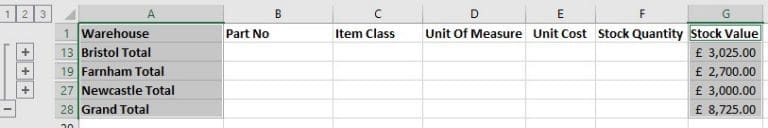
Excel Charts - Creating from Data Subtotals Sheet | JPL Derbyshire & UK
Solved: Show data label only to one line - Microsoft Power ... 1. Creating a separate measure for each item in your legend, like calculate (, [legendcolumn] = "legend value") 2. Remove the legend and the current measure from the line chart. 3. Add all of the measures to the line chart. 4. Then Data Labels will have the Customize Series option. View solution in original post.

How to Represent Data with a Pie of Pie Chart in Your Excel Worksheet - Data Recovery Blog
Only Display Some Labels On Pie Chart - Excel Help Forum Hi All, I have a pie chart that contains over 50 categories (Yes, I know pie charts shouldn't be used for that many things) but I want to only display labels for maybe the top 5 values or any label with a value >10. This is because there are a few standout values but I want all the other values to remain in the chart as it keeps the size of the larger values in context, i just dont want this ...

How to Add Filter to Pivot Table: 7 Steps (with Pictures)
Excel tutorial: How to use data labels Generally, the easiest way to show data labels to use the chart elements menu. When you check the box, you'll see data labels appear in the chart. If you have more than one data series, you can select a series first, then turn on data labels for that series only. You can even select a single bar, and show just one data label.

Add or remove data labels in a chart Click the data series or chart. To label one data point, after clicking the series, click that data point. In the upper right corner, next to the chart, click Add Chart Element > Data Labels. To change the location, click the arrow, and choose an option. If you want to show your data label inside a text bubble shape, click Data Callout.

excel - How do I update the data label of a chart? - Stack Overflow
support.microsoft.com › en-us › officeUpdate the data in an existing chart - support.microsoft.com Tip: To vary the color by data point in a chart that has only one data series, click the series, and then click the Format tab. Click Fill, and then depending on the chart, select the Vary color by point check box or the Vary color by slice check box. Depending on the chart type, some options may not be available.
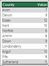
Create a Map Chart - Office Support
› office-addins-blog › 2018/10/10Find, label and highlight a certain data point in Excel ... Oct 10, 2018 · Click the Chart Elements button. Select the Data Labels box and choose where to position the label. By default, Excel shows one numeric value for the label, y value in our case. To display both x and y values, right-click the label, click Format Data Labels…, select the X Value and Y value boxes, and set the Separator of your choosing:

Enable or Disable Excel Data Labels at the click of a button - How To - PakAccountants.com
› 2015/11/12 › make-pie-chart-excelHow to make a pie chart in Excel Nov 12, 2015 · Adding data labels to Excel pie charts. In this pie chart example, we are going to add labels to all data points. To do this, click the Chart Elements button in the upper-right corner of your pie graph, and select the Data Labels option. Additionally, you may want to change the Excel pie chart labels location by clicking the arrow next to Data ...

Excel chart not printing correctly - i have a simple excel file (office
How to hide zero data labels in chart in Excel? Sometimes, you may add data labels in chart for making the data value more clearly and directly in Excel. But in some cases, there are zero data labels in the chart, and you may want to hide these zero data labels. Here I will tell you a quick way to hide the zero data labels in Excel at once. Hide zero data labels in chart

Charts In Excel – Excel Tutorial World
Display every "n" th data label in graphs - Microsoft ... you can use a free tool created by Rob Bovey, called the XY Chart Labeler. With this tool you can assign a range of cells to be the labels for chart series, instead of the Excel defaults. Using a formula, you can have a text show up in every nth cell and then use that range with the XY Chart Labeler to display as the series label.

show only specific data labels on the x-axis (category ... Say I only want to show the 2nd, 4th and 5th date on the x-axis. Is it possible to "turn-off" the rest of the text on the x-axis. It seems that excel treats the x-axis as a whole (a category axis object) and doesn't allow you to change the attributes of it's "sub-objects" such as the text of the 2nd, 4th and 5th data points.

Filtering charts in Excel - Microsoft 365 Blog The on-object chart controls in Excel allow you to quickly filter out data at the chart level, and filtering data here will only affect the chart—not the data. Select the chart, then click the Filter icon to expose the filter pane. From here, you can filter both series and categories directly in the chart. For example, hover over Fruit Pear ...

How to Add Data Labels to an Excel 2010 Chart - dummies
Is there a way to show only specific values in x-axis of ... 2. This question does not show any research effort; it is unclear or not useful. Bookmark this question. Show activity on this post. In my problem, I have 0.1 0.2 0.5 1.0 on the x-axis and I want to plot my chart by showing only these values on the horizontal-axis. Is there anyway or any extension (like kutools) to make this happen in Excel?

How to Create a Chart in Microsoft Excel - TechSupport
Label Specific Excel Chart Axis Dates - My Online Training Hub Step 1 - Insert a regular line or scatter chart. I'm going to insert a scatter chart so I can show you another trick most people don't know*. Step 2 - Hide the line for the 'Date Label Position' series: Step 3 - Set the desired minimum and maximum dates (Scatter Charts Only)

Excel Charts Archives - PakAccountants.com
Change the format of data labels in a chart To get there, after adding your data labels, select the data label to format, and then click Chart Elements > Data Labels > More Options. To go to the appropriate area, click one of the four icons ( Fill & Line, Effects, Size & Properties ( Layout & Properties in Outlook or Word), or Label Options) shown here.
Fixing Your Excel Chart When the Multi-Level Category Label Option is Missing. - Excel Dashboard ...
Add a DATA LABEL to ONE POINT on a chart in Excel | Excel ... Steps shown in the video above: Click on the chart line to add the data point to. All the data points will be highlighted. Click again on the single point that you want to add a data label to. Right-click and select ' Add data label ' This is the key step! Right-click again on the data point itself (not the label) and select ' Format data label '.

Doing Economics: Empirical Project 4: Working in Excel
Excel Chart - Do not Hide Horizontal Data Label - Stack ... 1) You can't see all your data labels on the X axis unless you format the X axis to have major interval of 1. 2) With a scatter plot, you cannot have your original labels retained on the X axis and, in your case, as your dates are recognised , they are ordered as such.
Post a Comment for "41 excel chart only show certain data labels"