42 excel graph data labels

How to Add Labels to Scatterplot Points in Excel - Statology Next, click anywhere on the chart until a green plus (+) sign appears in the top right corner. Then click Data Labels, then click More Options… In the Format Data Labels window that appears on the right of the screen, uncheck the box next to Y Value and check the box next to Value From Cells. Move data labels - support.microsoft.com Right-click the selection > Chart Elements > Data Labels arrow, and select the placement option you want. Different options are available for different chart types. For example, you can place data labels outside of the data points in a pie chart but not in a column chart.

Excel Charts - Aesthetic Data Labels - tutorialspoint.com To place the data labels in the chart, follow the steps given below. Step 1 − Click the chart and then click chart elements. Step 2 − Select Data Labels. Click to see the options available for placing the data labels. Step 3 − Click Center to place the data labels at the center of the bubbles. Format a Single Data Label

Excel graph data labels

Add / Move Data Labels in Charts - Excel & Google Sheets Adding Data Labels Click on the graph Select + Sign in the top right of the graph Check Data Labels Change Position of Data Labels Click on the arrow next to Data Labels to change the position of where the labels are in relation to the bar chart Final Graph with Data Labels How to Add Total Data Labels to the Excel Stacked Bar Chart 03/04/2013 · Step 4: Right click your new line chart and select “Add Data Labels” Step 5: Right click your new data labels and format them so that their label position is “Above”; also make the labels bold and increase the font size. Step 6: Right click the line, select “Format Data Series”; in the Line Color menu, select “No line” How to create Custom Data Labels in Excel Charts - Efficiency 365 Create the chart as usual. Add default data labels. Click on each unwanted label (using slow double click) and delete it. Select each item where you want the custom label one at a time. Press F2 to move focus to the Formula editing box. Type the equal to sign. Now click on the cell which contains the appropriate label.

Excel graph data labels. How to I rotate data labels on a column chart so that they are ... To change the text direction, first of all, please double click on the data label and make sure the data are selected (with a box surrounded like following image). Then on your right panel, the Format Data Labels panel should be opened. Go to Text Options > Text Box > Text direction > Rotate How to Rename a Data Series in Microsoft Excel - How-To Geek 27/07/2020 · A data series in Microsoft Excel is a set of data, shown in a row or a column, which is presented using a graph or chart. To help analyze your data, you might prefer to rename your data series. Rather than renaming the individual column or row labels, you can rename a data series in Excel by editing the graph or chart. Excel Graph Data Labels - Mouse Over Effects - Microsoft Community Excel; Microsoft 365 and Office; Search Community member; DB. Dyllan B. ... no, data labels in a chart will either be visible or not. A data point in a chart will show a pop up with information about the data point when the mouse is hovering over it, though. _____ cheers, teylyn ... How to Use Cell Values for Excel Chart Labels - How-To Geek Select the chart, choose the "Chart Elements" option, click the "Data Labels" arrow, and then "More Options." Uncheck the "Value" box and check the "Value From Cells" box. Select cells C2:C6 to use for the data label range and then click the "OK" button. The values from these cells are now used for the chart data labels.

How to Place Labels Directly Through Your Line Graph in Microsoft Excel ... Click on Add Data Labels. Your unformatted labels will appear to the right of each data point: Click just once on any of those data labels. You'll see little squares around each data point. Then, right-click on any of those data labels. You'll see a pop-up menu. Select Format Data Labels. In the Format Data Labels editing window, adjust the ... Excel Chart Data Labels - Microsoft Community Right-click a data point on your chart, from the context menu choose Format Data Labels ..., choose Label Options > Label Contains Value from Cells > Select Range. In the Data Label Range dialog box, verify that the range includes all 26 cells. When I paste your data into a worksheet, the XY Scatter data is in A2:B27, and the data labels are in ... How To Plot X Vs Y Data Points In Excel | Excelchat Figure 6 – Plot chart in Excel. If we add Axis titles to the horizontal and vertical axis, we may have this; Figure 7 – Plotting in Excel. Add Data Labels to X and Y Plot. We can also add Data Labels to our plot. These data labels can give us a clear idea of each data point without having to reference our data table. We can click on the ... › how-to-create-excel-pie-chartsHow to Make a Pie Chart in Excel & Add Rich Data Labels to ... Sep 08, 2022 · They are some of the most used chart types in reports, dashboards, and infographics. Excel provides a way to not only create charts but also to format them extensively so that they can be utilized with ease in presentations, posters and infographics. One can add rich data labels to data points or one point solely of a chart.

Add data labels and callouts to charts in Excel 365 - EasyTweaks.com The steps that I will share in this guide apply to Excel 2021 / 2019 / 2016. Step #1: After generating the chart in Excel, right-click anywhere within the chart and select Add labels . Note that you can also select the very handy option of Adding data Callouts. blog.hubspot.com › marketing › excel-graph-tricks-list10 Design Tips to Create Beautiful Excel Charts and Graphs in ... Sep 24, 2015 · To order the graphs in Excel, you'll need to sort the data from largest to smallest. Click 'Data,' choose 'Sort,' and select how you'd like to sort everything. 3) Shorten Y-axis labels. Long Y-axis labels, like large number values, take up a lot of space and can look a little messy, like in the chart below: Find, label and highlight a certain data point in Excel scatter graph 10/10/2018 · Select the Data Labels box and choose where to position the label. By default, Excel shows one numeric value for the label, y value in our case. To display both x and y values, right-click the label, click Format Data Labels…, select the X Value and Y value boxes, and set the Separator of your choosing: Label the data point by name how to add data labels into Excel graphs - storytelling with data You can download the corresponding Excel file to follow along with these steps: Right-click on a point and choose Add Data Label. You can choose any point to add a label—I'm strategically choosing the endpoint because that's where a label would best align with my design. Excel defaults to labeling the numeric value, as shown below.

Add data labels to your Excel bubble charts | TechRepublic

Transpose (rotate) data from rows to columns or vice versa Note: If your data is in an Excel table, the Transpose feature won’t be available. You can convert the table to a range first, or you can use the TRANSPOSE function to rotate the rows and columns. Here’s how to do it: Select the range of data you want to rearrange, including any row or column labels, and press Ctrl+C.

How-to Use Data Labels from a Range in an Excel Chart - Excel ...

Data Labels in Excel Pivot Chart (Detailed Analysis) 7 Suitable Examples with Data Labels in Excel Pivot Chart Considering All Factors 1. Adding Data Labels in Pivot Chart 2. Set Cell Values as Data Labels 3. Showing Percentages as Data Labels 4. Changing Appearance of Pivot Chart Labels 5. Changing Background of Data Labels 6. Dynamic Pivot Chart Data Labels with Slicers 7.

Adding rich data labels to charts in Excel 2013 | Microsoft ...

ExcelScript.ChartDataLabels interface - Office Scripts Methods. get Auto Text () Specifies if data labels automatically generate appropriate text based on context. get Format () Specifies the format of chart data labels, which includes fill and font formatting. get Horizontal Alignment () Specifies the horizontal alignment for chart data label. See ExcelScript.ChartTextHorizontalAlignment for details.

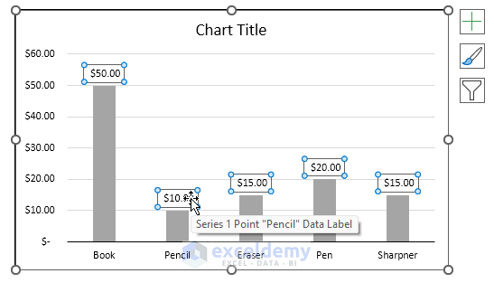
data visualization - How do you put values over a simple bar ...

› 682077 › how-to-rename-a-dataHow to Rename a Data Series in Microsoft Excel - How-To Geek Jul 27, 2020 · A data series in Microsoft Excel is a set of data, shown in a row or a column, which is presented using a graph or chart. To help analyze your data, you might prefer to rename your data series. Rather than renaming the individual column or row labels, you can rename a data series in Excel by editing the graph or chart.

Using the CONCAT function to create custom data labels for an ...

How To Use Dynamic Data Labels To Create Interactive Excel Charts Insert An Interactive Line Chart With Dynamic Data Labels. Select the data and insert a combo chart. For combo, chart go to the Insert → Charts → Combo Charts. Now make a selection for the Line Chart for revenue data and a Line Chart With Markers For Data Labels. Now select the Data Label Line and remove fill color from it.

Highlight a Specific Data Label in an Excel Chart - Peltier Tech

How to Add Data Labels to an Excel 2010 Chart - dummies On the Chart Tools Layout tab, click Data Labels→More Data Label Options. The Format Data Labels dialog box appears. You can use the options on the Label Options, Number, Fill, Border Color, Border Styles, Shadow, Glow and Soft Edges, 3-D Format, and Alignment tabs to customize the appearance and position of the data labels.

Area Chart Data Label | MrExcel Message Board

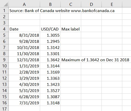
How to add a line in Excel graph: average line, benchmark, etc. The label will appear at the end of the line giving more information to your chart viewers: Add a text label for the line. To improve your graph further, you may wish to add a text label to the line to indicate what it actually is. ... I have multiple data and i draw a excel graph. My X axis vales are 10, 20 30 , 40 and corresponding Y axis ...

Custom Data Labels with Colors and Symbols in Excel Charts ...

› office-addins-blog › 2018/10/10Find, label and highlight a certain data point in Excel ... Here's how: Click on the highlighted data point to select it. Click the Chart Elements button. Select the Data Labels box and choose where to position the label. By default, Excel shows one numeric value for the label, y value in our case. To display both x and y values, right-click the label, click Format Data Labels…, select the X Value and ...

How to Place Labels Directly Through Your Line Graph in ...

How to add data labels from different column in an Excel chart? This method will introduce a solution to add all data labels from a different column in an Excel chart at the same time. Please do as follows: 1. Right click the data series in the chart, and select Add Data Labels > Add Data Labels from the context menu to add data labels. 2.

Enable or Disable Excel Data Labels at the click of a button ...

Add or remove data labels in a chart - Microsoft Support Add data labels to a chart Click the data series or chart. To label one data point, after clicking the series, click that data point. In the upper right corner, next to the chart, click Add Chart Element > Data Labels. To change the location, click the arrow, and choose an option.

Custom data labels in a chart

Custom Chart Data Labels In Excel With Formulas - How To Excel At Excel Follow the steps below to create the custom data labels. Select the chart label you want to change. In the formula-bar hit = (equals), select the cell reference containing your chart label's data. In this case, the first label is in cell E2. Finally, repeat for all your chart laebls.

Format Data Labels in Excel- Instructions - TeachUcomp, Inc.

How to Add Data Labels in Excel - Excelchat | Excelchat After inserting a chart in Excel 2010 and earlier versions we need to do the followings to add data labels to the chart; Click inside the chart area to display the Chart Tools. Figure 2. Chart Tools Click on Layout tab of the Chart Tools. In Labels group, click on Data Labels and select the position to add labels to the chart. Figure 3.

microsoft excel - Prevent two sets of labels from overlapping ...

How to Make a Pie Chart in Excel & Add Rich Data Labels to 08/09/2022 · A pie chart is used to showcase parts of a whole or the proportions of a whole. There should be about five pieces in a pie chart if there are too many slices, then it’s best to use another type of chart or a pie of pie chart in order to showcase the data better. In this article, we are going to see a detailed description of how to make a pie chart in excel.

Align data labels in a graph so they are all along the same ...

› solutions › excel-chatHow To Plot X Vs Y Data Points In Excel | Excelchat Figure 6 – Plot chart in Excel. If we add Axis titles to the horizontal and vertical axis, we may have this; Figure 7 – Plotting in Excel. Add Data Labels to X and Y Plot. We can also add Data Labels to our plot. These data labels can give us a clear idea of each data point without having to reference our data table. We can click on the ...

How to add or move data labels in Excel chart?

How to Change Excel Chart Data Labels to Custom Values? - Chandoo.org First add data labels to the chart (Layout Ribbon > Data Labels) Define the new data label values in a bunch of cells, like this: Now, click on any data label. This will select "all" data labels. Now click once again. At this point excel will select only one data label. Go to Formula bar, press = and point to the cell where the data label ...

Two-Level Axis Labels (Microsoft Excel)

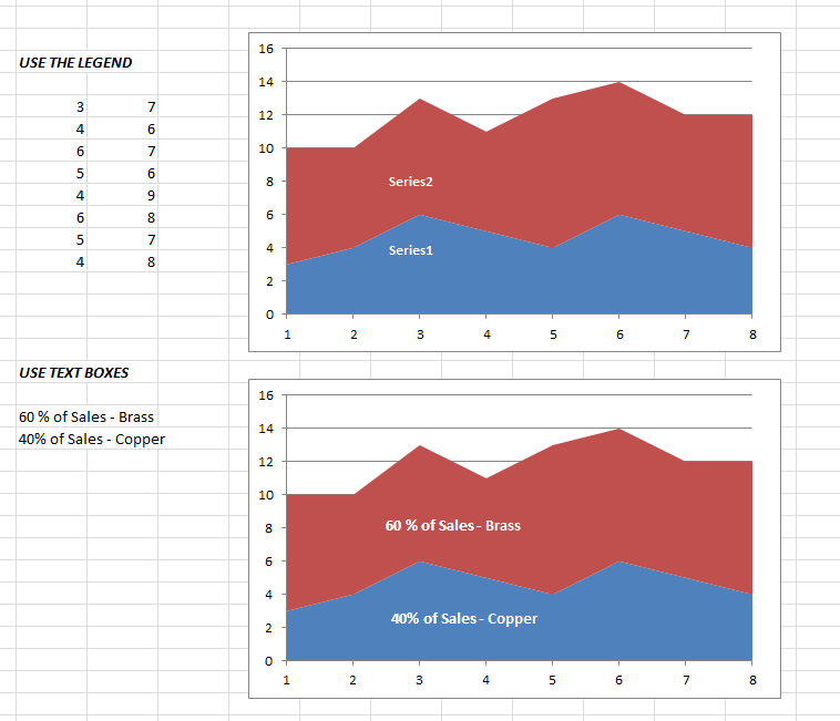
› excel › how-to-add-total-dataHow to Add Total Data Labels to the Excel Stacked Bar Chart Apr 03, 2013 · Step 4: Right click your new line chart and select “Add Data Labels” Step 5: Right click your new data labels and format them so that their label position is “Above”; also make the labels bold and increase the font size. Step 6: Right click the line, select “Format Data Series”; in the Line Color menu, select “No line”

Add / Move Data Labels in Charts – Excel & Google Sheets ...

Change the format of data labels in a chart To get there, after adding your data labels, select the data label to format, and then click Chart Elements > Data Labels > More Options. To go to the appropriate area, click one of the four icons ( Fill & Line, Effects, Size & Properties ( Layout & Properties in Outlook or Word), or Label Options) shown here.

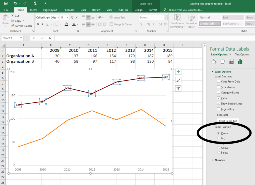
How to Place Labels Directly Through Your Line Graph in ...

Add a DATA LABEL to ONE POINT on a chart in Excel Steps shown in the video above: Click on the chart line to add the data point to. All the data points will be highlighted. Click again on the single point that you want to add a data label to. Right-click and select ' Add data label ' This is the key step! Right-click again on the data point itself (not the label) and select ' Format data label '.

how to add data labels into Excel graphs — storytelling with data

Edit titles or data labels in a chart - support.microsoft.com The first click selects the data labels for the whole data series, and the second click selects the individual data label. Right-click the data label, and then click Format Data Label or Format Data Labels. Click Label Options if it's not selected, and then select the Reset Label Text check box. Top of Page

How to avoid data label in excel line chart overlap with ...

› documents › excelHow to add data labels from different column in an Excel chart? This method will introduce a solution to add all data labels from a different column in an Excel chart at the same time. Please do as follows: 1. Right click the data series in the chart, and select Add Data Labels > Add Data Labels from the context menu to add data labels. 2.

Excel Charts - Aesthetic Data Labels

3 Types of Line Graph/Chart: + [Examples & Excel Tutorial] 20/04/2020 · See the sample data below and follow these simple steps when creating a line graph for your data. Create and Format Data For Line Graph. When creating a line chart, you need to have a horizontal (x) axis and a vertical (y) axis. Therefore, when entering your data on the Excel worksheet, you need to indicate these axes by creating 2 columns.

Add or remove data labels in a chart

How to Use Cell Values for Excel Chart Labels - How-To Geek 12/03/2020 · Make your chart labels in Microsoft Excel dynamic by linking them to cell values. When the data changes, the chart labels automatically update. In this article, we explore how to make both your chart title and the chart data labels dynamic. We have the sample data below with product sales and the difference in last month’s sales.

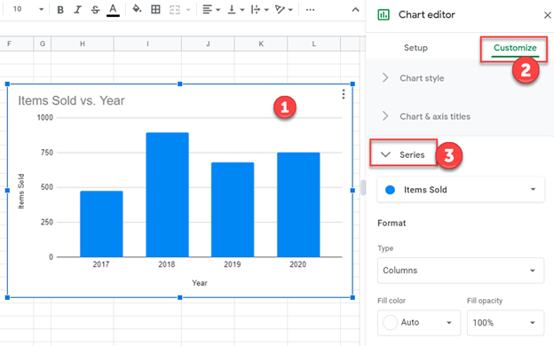
Google Workspace Updates: Get more control over chart data ...

Excel tutorial: How to use data labels Generally, the easiest way to show data labels to use the chart elements menu. When you check the box, you'll see data labels appear in the chart. If you have more than one data series, you can select a series first, then turn on data labels for that series only. You can even select a single bar, and show just one data label.

264. How can I make an Excel chart refer to column or row ...

10 Design Tips to Create Beautiful Excel Charts and Graphs in … 24/09/2015 · To order the graphs in Excel, you'll need to sort the data from largest to smallest. Click 'Data,' choose 'Sort,' and select how you'd like to sort everything. 3) Shorten Y-axis labels. Long Y-axis labels, like large number values, take up a lot of space and can look a little messy, like in the chart below:

Change the format of data labels in a chart

How to add or move data labels in Excel chart? - ExtendOffice In Excel 2013 or 2016. 1. Click the chart to show the Chart Elements button . 2. Then click the Chart Elements, and check Data Labels, then you can click the arrow to choose an option about the data labels in the sub menu. See screenshot: In Excel 2010 or 2007. 1. click on the chart to show the Layout tab in the Chart Tools group. See ...

Adding rich data labels to charts in Excel 2013 | Microsoft ...

How to create Custom Data Labels in Excel Charts - Efficiency 365 Create the chart as usual. Add default data labels. Click on each unwanted label (using slow double click) and delete it. Select each item where you want the custom label one at a time. Press F2 to move focus to the Formula editing box. Type the equal to sign. Now click on the cell which contains the appropriate label.

How to fix wrapped data labels in a pie chart | Sage Intelligence

How to Add Total Data Labels to the Excel Stacked Bar Chart 03/04/2013 · Step 4: Right click your new line chart and select “Add Data Labels” Step 5: Right click your new data labels and format them so that their label position is “Above”; also make the labels bold and increase the font size. Step 6: Right click the line, select “Format Data Series”; in the Line Color menu, select “No line”