42 format data labels pane excel

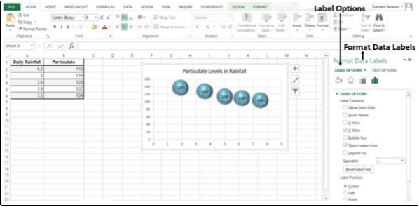
› documents › excelHow to add data labels from different column in an Excel chart? In the Format Data Labels pane, under Label Options tab, check the Value From Cells option, select the specified column in the popping out dialog, and click the OK button. Now the cell values are added before original data labels in bulk. 4. Go ahead to untick the Y Value option (under the Label Options tab) in the Format Data Labels pane. How to Create Mailing Labels in Excel - Excelchat Figure 26 - Print labels from excel (If we click No, Word will break the connection between document and Excel data file.) C. Alternatively, we can save merged labels as usual text. When we use this format, Excel will save our labels as a normal word document without linking to the Excel source file.

Adding rich data labels to charts in Excel 2013 ... Basic formatting of data labels is simple to achieve by using the Font section of the Home tab on the Excel ribbon. Use the Formatting Task pane for advanced options If you wish to go beyond basic text formatting and text box fills, many more formatting options are available on the Formatting Task pane.

Format data labels pane excel

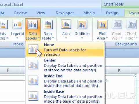
How to Add Data Labels to an Excel 2010 Chart - dummies On the Chart Tools Layout tab, click Data Labels→More Data Label Options. The Format Data Labels dialog box appears. You can use the options on the Label Options, Number, Fill, Border Color, Border Styles, Shadow, Glow and Soft Edges, 3-D Format, and Alignment tabs to customize the appearance and position of the data labels. › make-labels-with-excel-4157653How to Print Labels from Excel - Lifewire Select Mailings > Write & Insert Fields > Update Labels . Once you have the Excel spreadsheet and the Word document set up, you can merge the information and print your labels. Click Finish & Merge in the Finish group on the Mailings tab. Click Edit Individual Documents to preview how your printed labels will appear. Select All > OK . Excel Charts - Quick Formatting - Tutorialspoint Excel Charts - Quick Formatting. You can format charts quickly using the Format pane. It is quite handy and provides advanced formatting options. Step 1 − Click on the chart. Step 2 − Right-click chart element. Step 3 − Click Format from the drop-down list. The Format pane appears with options that are tailored for the ...

Format data labels pane excel. 2/ Right-click i.e. on the 1st histo. bar (A) > Add Data Labels (numbers are displayed a the top of the bars) 3/ Click one of the numbers that just displayed (the Format Data Labels pane opens on the right) > Check option "Value From Cells" > Select range C2:C7 > OK > Uncheck option "Value" demo.png (18.5 KiB) · 3 Creating Pie Chart and Adding/Formatting Data Labels (Excel) Creating Pie Chart and Adding/Formatting Data Labels (Excel) Excel Charts - Aesthetic Data Labels - Tutorialspoint To format the data labels − Step 1 − Right-click a data label and then click Format Data Label. The Format Pane - Format Data Label appears. Step 2 − Click the Fill & Line icon. The options for Fill and Line appear below it. Step 3 − Under FILL, Click Solid Fill and choose the color. How to Customize Your Excel Pivot Chart Data Labels - dummies To remove the labels, select the None command. If you want to specify what Excel should use for the data label, choose the More Data Labels Options command from the Data Labels menu. Excel displays the Format Data Labels pane. Check the box that corresponds to the bit of pivot table or Excel table information that you want to use as the label.

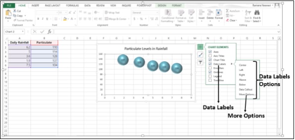
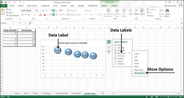
How to add or move data labels in Excel chart? 2. Then click the Chart Elements, and check Data Labels, then you can click the arrow to choose an option about the data labels in the sub menu. See screenshot: In Excel 2010 or 2007. 1. click on the chart to show the Layout tab in the Chart Tools group. See screenshot: 2. Then click Data Labels, and select one type of data labels as you need ... Excel tutorial: The Format Task pane You can also select a chart element first, then use the keyboard shortcut Control + 1. For example, if I select the data bars in this chart, then type Control + 1, the Format Task Pane will open with with the data series options selected. The Format Task pane stays open until you manually close the window. Format a Map Chart - support.microsoft.com Formatting Guidelines. Following are some guidelines for formatting a Map chart's Series Options.To display the Series Options for your map chart you can right-click on the outer portion of the map and select Format Chart Area in the right-click menu, or double-click on the outer portion of the map. You should see the Format Object Task Pane on the right-hand side of the Excel window. How do you format data series in Excel? - faq-all.com To format data labels in EÎl , choose the set of data labels to format . To do this, click the " Format " tab within the "Chart Tools" contextual tab in the Ribbon. Then select the data labels to format from the "Chart Elements" drop-down in the "Current Selection" button group. How do I show the Format Data Series pane in Excel?

› make-chart-x-axis-labelsMake Chart X Axis Labels Display below Negative Data - Excel How Aug 21, 2018 · #2 right click on the selected X Axis, and select Format Axis… from the pop-up menu list. The Format Axis pane will be displayed in the right of excel window. #3 on Format Axis pane, expand the Labels section, select Low option from the Label Position drop-down list box. Close the Format Axis pane. How to Print Labels From Excel - EDUCBA Navigate towards the folder where the excel file is stored in the Select Data Source pop-up window. Select the file in which the labels are stored and click Open. A new pop up box named Confirm Data Source will appear. Click on OK to let the system know that you want to use the data source. Again a pop-up window named Select Table will appear. Edit titles or data labels in a chart - support.microsoft.com The first click selects the data labels for the whole data series, and the second click selects the individual data label. Right-click the data label, and then click Format Data Label or Format Data Labels. Click Label Options if it's not selected, and then select the Reset Label Text check box. Top of Page Format elements of a chart - support.microsoft.com Right-click the chart axis, and click Format Axis. In the Format Axis task pane, make the changes you want. You can move or resize the task pane to make working with it easier. Click the chevron in the upper right. Select Move and then drag the pane to a new location. Select Size and drag the edge of the pane to resize it.

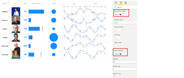
Multiple Sparklines – Power BI & Excel are better together

support.microsoft.com › en-us › officeChange the format of data labels in a chart To get there, after adding your data labels, select the data label to format, and then click Chart Elements > Data Labels > More Options. To go to the appropriate area, click one of the four icons ( Fill & Line , Effects , Size & Properties ( Layout & Properties in Outlook or Word), or Label Options ) shown here.

» Excel Charts: Creating Custom Data Labels

› format-data-labels-in-excelFormat Data Labels in Excel- Instructions - TeachUcomp, Inc. Nov 14, 2019 · Alternatively, you can right-click the desired set of data labels to format within the chart. Then select the “Format Data Labels…” command from the pop-up menu that appears to format data labels in Excel. Using either method then displays the “Format Data Labels” task pane at the right side of the screen. Format Data Labels in Excel ...

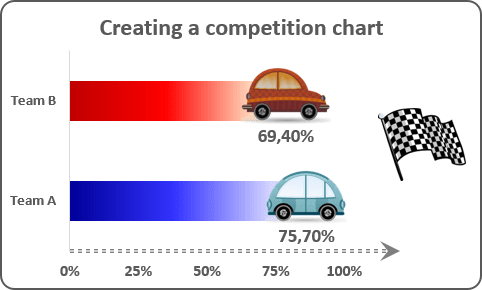
Creating a simple competition chart

excelunlocked.com › format-chart-axis-in-excelFormat Chart Axis in Excel – Axis Options Dec 14, 2021 · Axis Options : Number Format. We can change the format of axis values of the chart in excel in the same way we do for the cell entries. Below are the number formats available for chart values in excel. It is currently set to general number format. We would choose the currency from the list.

Create a slider bead chart in Excel

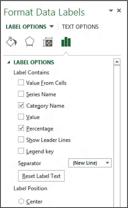
Excel tutorial: How to use data labels When first enabled, data labels will show only values, but the Label Options area in the format task pane offers many other settings. You can set data labels to show the category name, the series name, and even values from cells. In this case for example, I can display comments from column E using the "value from cells" option.

Directly Labeling Excel Charts - Policy Viz

Use custom formats in an Excel chart's axis and data labels Choose Number in the left pane. (In Excel 2003, click the Number tab.) ... Right-click a series and choose Format Data Labels from the context menu. If you don't see that option, right-click ...

How to add data labels to a chart in a spreadsheet - YouTube

support.microsoft.com › en-us › officePrepare your Excel data source for a Word mail merge In your Excel data source that you'll use for a mailing list in a Word mail merge, make sure you format columns of numeric data correctly. Format a column with numbers, for example, to match a specific category such as currency. If you choose percentage as a category, be aware that the percentage format will multiply the cell value by 100.

Chart Data Labels in PowerPoint 2013 for Windows

Custom data labels in a chart - Get Digital Help Press with mouse on "Add Data Labels". Press with mouse on Add Data Labels". Double press with left mouse button on any data label to expand the "Format Data Series" pane. Enable checkbox "Value from cells". A small dialog box prompts for a cell range containing the values you want to use a s data labels. Select the cell range and press with ...

Excel charts: add title, customize chart axis, legend and data labels

Format Data Label: Label Position - Microsoft Community when you add labels with the + button next to the chart, you can set the label position. In a stacked column chart the options look like this: For a clustered column chart, there is an additional option for "Outside End" When you select the labels and open the formatting pane, the label position is in the series format section. Does that help?

Data Callout Excel 2019 Mac - greenwaymedicine

How to hide zero data labels in chart in Excel? - ExtendOffice If you want to hide zero data labels in chart, please do as follow: 1. Right click at one of the data labels, and select Format Data Labels from the context menu. See screenshot: 2. In the Format Data Labels dialog, Click Number in left pane, then select Custom from the Category list box, and type #"" into the Format Code text box, and click Add button to add it to Type list box.

Advanced Excel - более богатые метки данных - CoderLessons.com

Add a DATA LABEL to ONE POINT on a chart in Excel You can now configure the label as required — select the content of the label (e.g. series name, category name, value, leader line), the position (right, left, above, below) in the Format Data Label pane/dialog box. To format the font, color and size of the label, now right-click on the label and select 'Font'. Note: in step 5. above, if ...

How to show percentages on three different charts in Excel - Excel Board

Add or remove data labels in a chart - support.microsoft.com Right-click the data series or data label to display more data for, and then click Format Data Labels. Click Label Options and under Label Contains, select the Values From Cells checkbox. When the Data Label Range dialog box appears, go back to the spreadsheet and select the range for which you want the cell values to display as data labels.

How to create a chart with both percentage and value in Excel?

Format Data Labels Task Pane Excel In the Chart Layouts group, select Add Chart Element > Data Labels > More Data Label Options This activates the Format Data Labels task pane. Under Label Contains, tick the check box Value From Cells. A dialog will pop up to let you specify the range to use. › Verified 3 days ago › Url: answers.microsoft.com Go Now

Change the format of data labels in a chart

Excel Charts - Quick Formatting - Tutorialspoint Excel Charts - Quick Formatting. You can format charts quickly using the Format pane. It is quite handy and provides advanced formatting options. Step 1 − Click on the chart. Step 2 − Right-click chart element. Step 3 − Click Format from the drop-down list. The Format pane appears with options that are tailored for the ...

Format Data Labels in Excel 2013- Tutorial - TeachUcomp, Inc.

› make-labels-with-excel-4157653How to Print Labels from Excel - Lifewire Select Mailings > Write & Insert Fields > Update Labels . Once you have the Excel spreadsheet and the Word document set up, you can merge the information and print your labels. Click Finish & Merge in the Finish group on the Mailings tab. Click Edit Individual Documents to preview how your printed labels will appear. Select All > OK .